South LA Crime Analysis

2020 · GIS, Web Scraping, Buffer Analysis, R

South LA revisited with an OLS, Elastic Net, and Random Forest Regression.

• Authors: Elmer Camargo, Nicholas Trella, Geoffrey Hughes, Alberto Ng

Motivation

The Tobacco Related Disease Research Program (TRDRP) funded Chapman University’s Crean College faculty Dr. Jason Douglas to continue a study in South Los Angeles pertaining to geography of crime surrounding nuisance properties in large urban low income communities of color (Subica et al., 2016). This paper identified key aspects of the problem space including: The community identification of nuisance properties to be tobacco shops, liquor stores, and marijuana dispensaries in South Los Angeles, the prevalence of nuisance properties and its ecological effects on crime and the community, and a theoretical framework outlining social disorganization to be a signal for a compromised system of social controls thus increasing risk of crime. The paper also conducts three statistical techniques to analyze crime, property types, and demographic data. A Kruskal Wallis H test comparing crime count means within buffers of nuisance properties and convenience stores, an ordinary least squares regression model predicting crime count within a census tract, and a geographic weighted regression model predicting crime count as well. Our study expands on the ordinary least squares regression model and includes an elastic net regression model and a random forest model and is updated for the year 2017 instead of 2014. Aside from the TRDRP stakeholders, beneficiaries from this study include: policy makers governing legislations, control boards, and zoning requirements, the community to push awareness of results, public health specialists to validate and expand on the study, and police forces to re-examine and focus efforts appropriately.

Data Sets

Our project makes use of a variety of datasets. Some are downloaded from government websites, and others we made ourselves using the Google Places API to scrape location data. The full extent of our datasets came from the US Census, LAPD Crime data, LASD Crime data, the Center for Disease Control, and finally a python script that uses the Google Places API to scrape data on key search terms. In order to scrape location data for all places like liquor stores, dispensaries, parks, tobacco shops, and any other search term, I wrote a script in python. It takes in an initial point as the center for the search in longitude and latitude, a radius in meters to define the area of interest around that center point, and a list of keywords to query Google Places within that area. What gets output is a CSV file for each keyword containing the place’s name, longitude, latitude, address, zip code, rating, and some other variables. We then make use of this geolocation data to correctly locate each place and figure out which census tract they are in. From there, we can manipulate and play with the data to find crime trends among census tracts with varying numbers of, say, liquor stores or community centers. Along with our other downloaded and cleaned datasets, we make use of this scraped data to build our model and find trends in South LA. This program is dynamic, and can further be used to find places relevant to the input search terms anywhere google maps has data.

Data Wrangling

Because our data came from a variety of sources, we applied a range of mutations and transformations in order to join our data into a single data frame. Census data had to be renamed and filtered down to only include South Los Angeles census tracts. Additional mutations were made thereafter to create a population density, community mobility, racial heterogeneity, and economic class variables. After the demographic mutations, crime and property type data points had to be joined to the South Los Angeles shapefile. To do so, we transformed the shapefile into a spatial feature and aggregated census tract sums for property and violent crime reports and property types. Following the spatial join, we used multivariate imputation via chained equations to predict and replace missing values in the mental and physical health variables.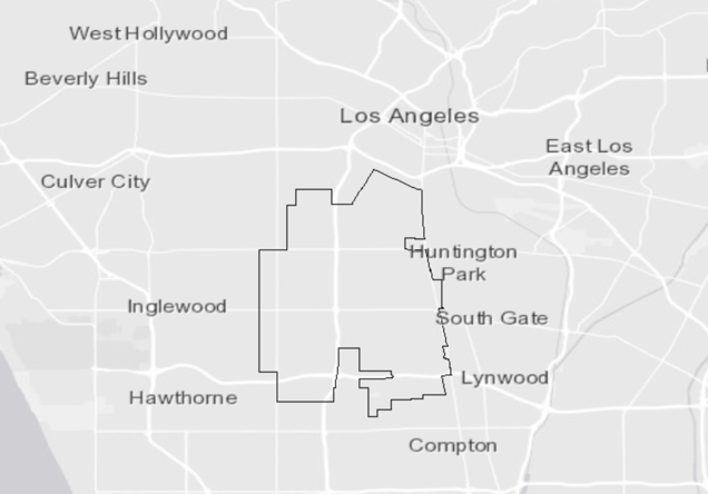

Summary Statistics

The South Los Angeles description from 2014 continues to hold valid from summary statistics in 2017. Hispanic and African American communities continue to be the predominant ethnicity group.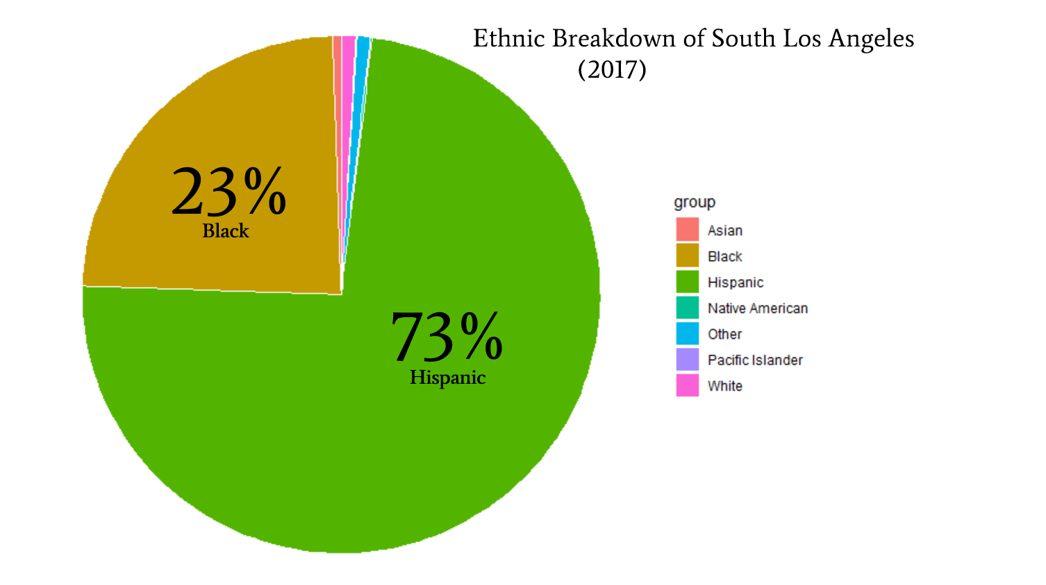
Economically, South LA is for the most part middle class earning between $25,000 to $75,000, and lower class <$10,000 to $24,999.
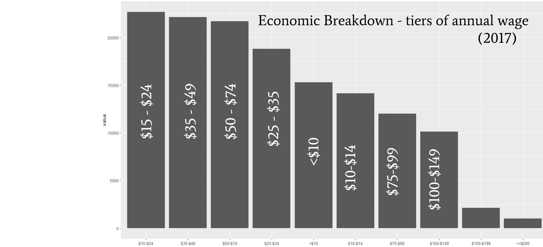From mapped variables, the north side of South LA is the most population dense likely due to the vicinity of the University of Southern California.
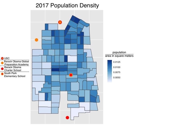Alternatively, the north seems to have to have a lower unemployment rate than the rest of South LA, again potentially due to the vicinity of the USC and potentially better economic infrastructure and job opportunity.
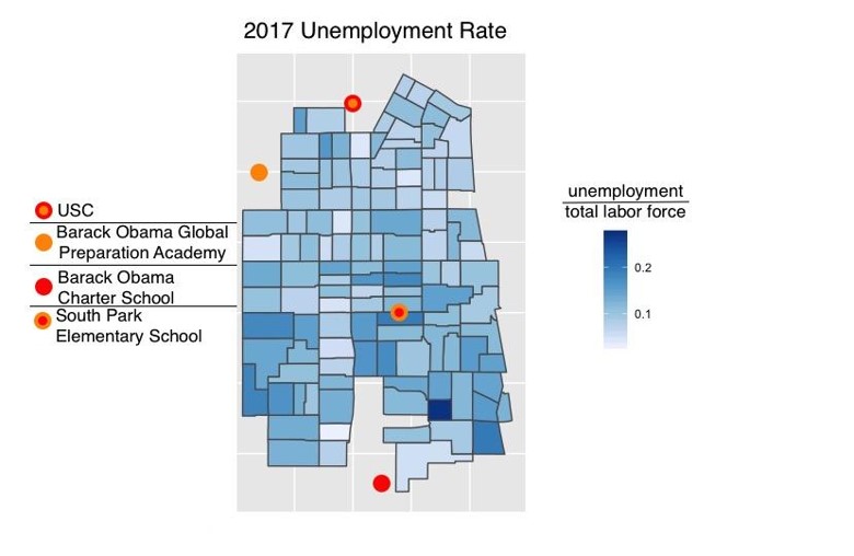Below poverty rates appear to be fairly spread out with the west side being slightly more poverty stricken.
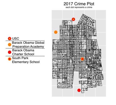
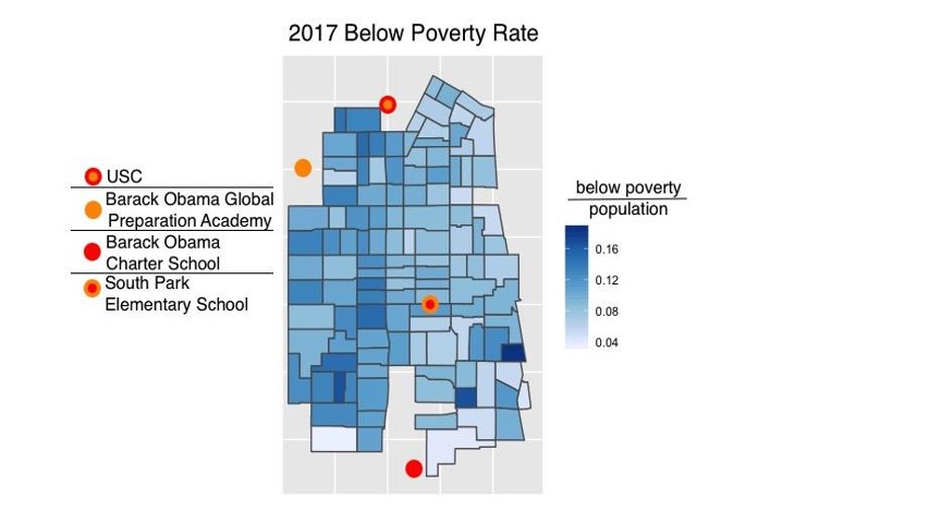Based off of publicly available data from the LAPD we were able to measure that reported crime in South LA steadily increased from 2010 to 2018 and reached a peak in 2017.
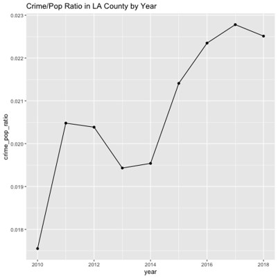Of these crimes larceny, narcotics related crime, and grand theft auto were the top three crimes in 2017 after crime data was reduced to only violent and property crimes.

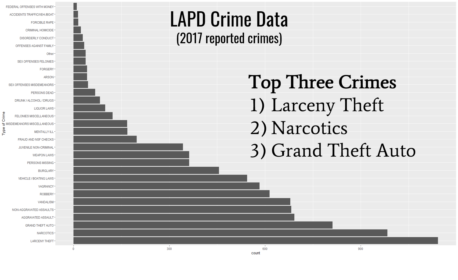
Regressions (OLS and Elastic Net)

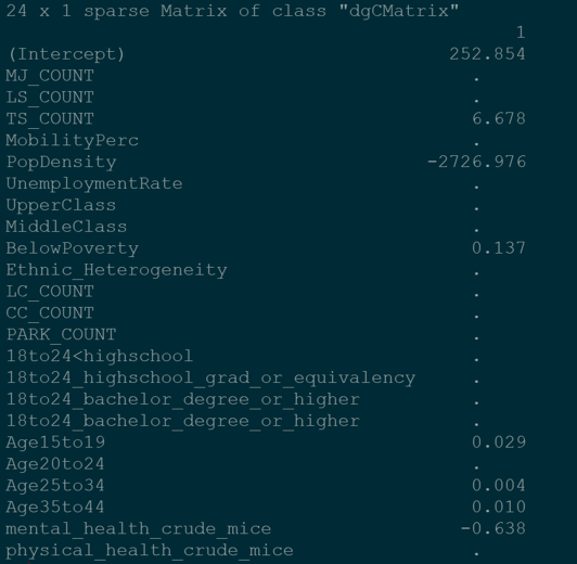
Given that crime count is continuous variable, we used an ordinary least squares regression model with nuisance property counts, community mobility, population density, unemployment rate, economic classes, racial heterogeneity, education levels, age, and physical and mental health as predictor variables. We also applied a training and test cross validation method to train our model on sixty percent of the census tracts and test on the remaining forty.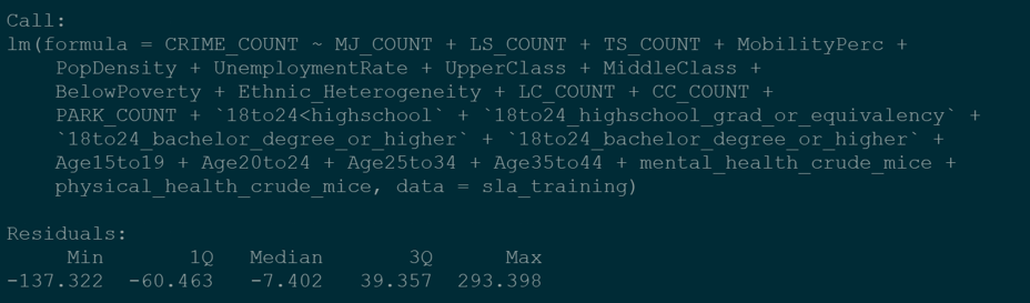
Doing so we calculated an R2 of .57 and an RMSE of 84.54 on the training set and an R2 of .39 and an RMSE of 82.79 on the test set. Variables displaying a p-value less than .05 included tobacco shops count, population density, below poverty count, and the imputed mental health estimate. We initially thought all variables would have a positive coefficient, however we were surprised to see that population density and the mental health estimates were negative. Population density we reasoned to have a negative impact on crime due to more people possibly dissuading criminal activity. The mental health estimate, we believe may have lost integrity after imputing missing values.

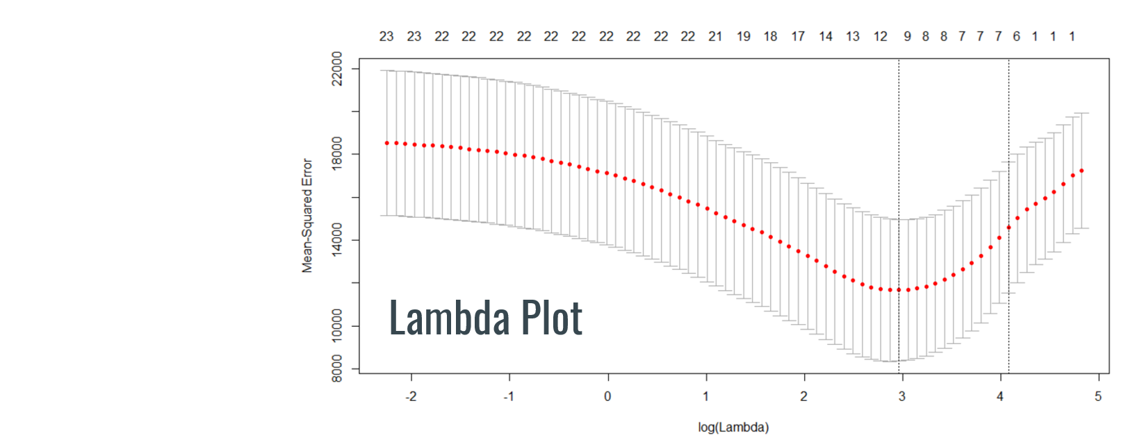
Although OLS provided suitable results we decided to use an elastic net model to validate findings. After elastic net alpha plotting we decided to use 0.5 as our hyperparameter so that we minimize cross validation loss and adjust for alpha penalization.

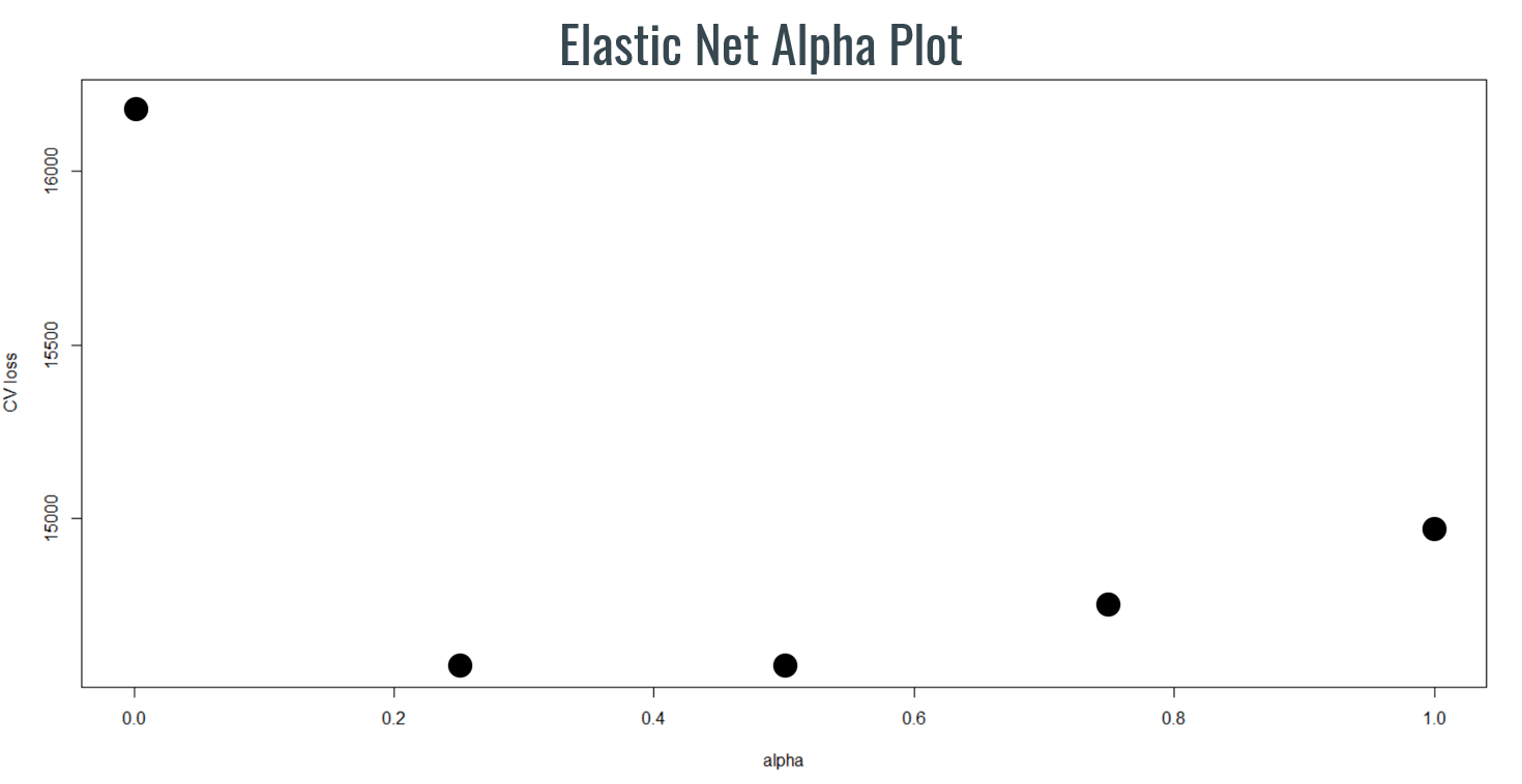
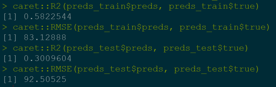
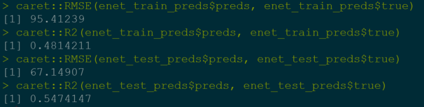
Some of the variables that were used were population density and education. With the results for RMSE and R2 for both the training set and test set, we can say that our model works better with test set, which we are happy to see. One interesting thing to point out is the population density has a big negative intercept which indicates a negative relationship. But with further thinking, we suspect this to either be a scaling issue on our hand or the student population in USC skewed the results.

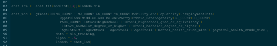
Random Forest

We then decided that although the results from the Elastic Net outperformed OLS, there may be an even further efficacy increase if we were to implement a random forest model. Essentially an amalgamation of many decision trees, we thought that the potential classification nature of crime estimation would lend itself well to this type of model. With there being so many potential factors in where crime is most prevalent having variables selected in order of importance and frequency through average node depth could paint a better picture on the key determinants of crime. Crime most certainly begets crime but there must be a myriad of other potential factors for such a complex social phenomenon. Our random forest model was set with 1000 trees as we found that beyond that the computational power needed did not justify the minimal error improvements. Past a few hundred trees is where most of the error reduction occurs.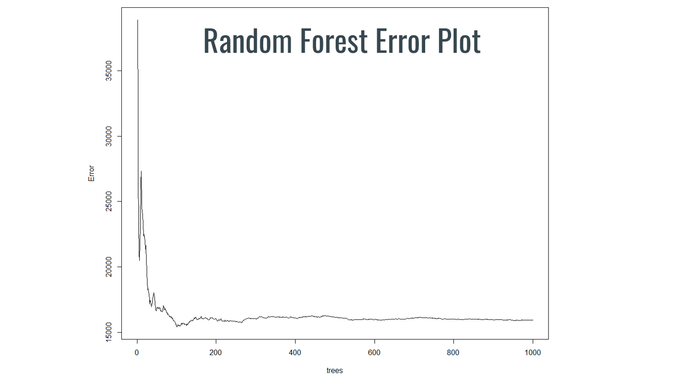

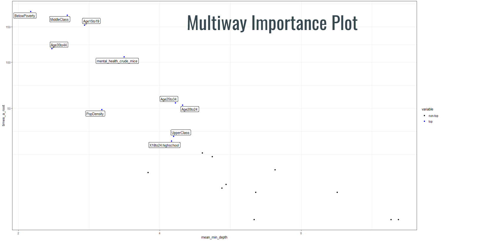Harkening back to our initial exploration of the data, the random forest node depth output seemed to be in line with something previously noted. Two variables stood out here, being classified as below poverty (less than 30 thousand USD annual household income) and population density. This seemed to make sense as the lack of a steady income, coupled with a lack of people would make committing a crime that much more attractive. In doing a cross-chart of these two variables to see crime count estimations as a function of them individually and them together we were able to see an observable correlation between the presence of poverty and lack of people as being key indicators of crime. Likewise, where many people and those people are not in poverty we see less occurrences of criminal activity.
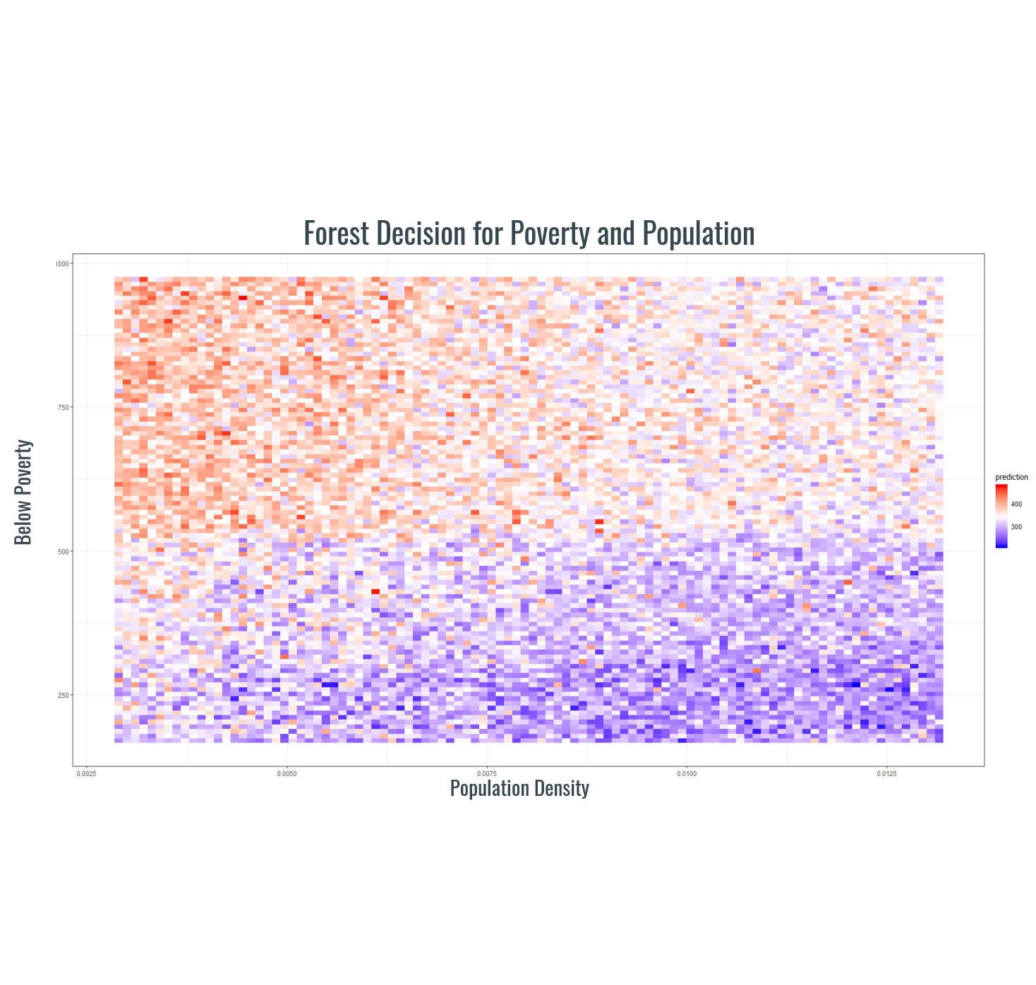Although our results seemed to paint a pretty decent picture of things to note by themselves it is hard to ascertain valuable information. We merely see a correlated impact between them without any say regarding the causality that may or may not be present. We’re quite confident that there is something about these two variables that have the observed impact however as it agrees with the previously established literature.

Conclusion

From our studies, we found results similar to that of the previous 2014 study leading us to agree with prior findings. Population density and high poverty count hold a strong magnitude in estimating crime within a census tract, and there is also significant probability that tobacco shops and census tract mental health may also play a role. Although these findings were found to be significant using ordinary least squares, elastic net, and random forest regression, we however need to research further into using Moran’s autocorrelation coefficient (Moran’s I Index) and using parametric heteroscedasticity and autocorrelation consistent standard errors (Conley Spatial HAC) in order to refine results. Accounting for spatial statistical factors would further prove our findings that tobacco shops are likely to be affecting crime, population dense census tracts have lower crime counts, and poverty increases crime. Mental health may also potentially play a role, however further research would have to be conducted to determine whether or not an imputation was useful for the regression models, and if so, further investigation for reasons why it had a negative impact on crime. Overall, models performed well given the complexity of the task. Moving forward with this research in the future will include an analysis of years between 2014-2018 as well as include comparisons of other cities.